ICEANS 2025 · 7th International Conference on Engineering and Applied Natural Sciences · Konya
Meta-Learner Ensemble Model for Brain Tumor Classification
Summary
At a Glance
Three pretrained CNNs look at the same MRI scan; a small MLP meta-learner learns how to combine their outputs into one of four classes: glioma, meningioma, pituitary tumor or no tumor.
Median blur, Otsu thresholding and cropping to the largest region focus the networks on the head.
A learned combiner instead of a fixed vote: it can trust each base model where it is strong.
Automatic mixed precision keeps training practical on a 6 GB laptop GPU.
I · Introduction
Why Automate Brain Tumor Classification?
- The tumor type guides treatment, so early and correct classification of MRI scans matters.
- Manual reading of many slices is time-consuming and prone to errors.
- Single CNNs already perform well; ensembles of several CNNs have pushed accuracy further in recent studies.
- Open problems: overfitting, limited or inconsistent datasets, and the computational cost of running several networks.
Arises from glial cells inside the brain tissue.
Grows from the meninges, the membranes around the brain.
Forms in the pituitary gland at the skull base.
I · Related Work · Interactive
Ensembles for Brain Tumor MRI
Results as reported by each study on its own data; not directly comparable. Click a column header to sort.
| Study | Ensemble | Data | Reported result | Ref. |
|---|---|---|---|---|
| Jader et al. | VGG-16, ResNet-50, AlexNet | 4 classes | 99.16% accuracy | 1 |
| Tandel et al. | 5 CNNs, majority vote | T1W, T2W, FLAIR glioma grading | up to 98.88% accuracy | 2 |
| Ghafourian et al. | Naive Bayes, SVM, KNN after spider-optimized segmentation | BRATS 2014, BTD20 | 98.61% / 99.13% accuracy | 3 |
| Anand et al. | VGG19 + CNN, weighted average | TCGA lower-grade glioma | reduced overfitting | 4 |
| Çetin-Kaya and Kaya | 5 CNNs weighted by particle swarm optimization | 3 datasets | up to 99.92% accuracy | 5 |
| Vaiyapuri et al. | EfficientNet, DenseNet, MobileNet + Gabor filter | BRATS 2015 | improved classification | 6 |
| Asif et al. | DenseNet201, ResNet152V2, InceptionResNetV2 (stacked) | Figshare | 98.69% accuracy | 7 |
| Hassan et al. | EL-APMC | BRATS 2015 glioma grades | 88.73% accuracy, 93.12% F1 | 8 |
| Kang et al. | VGG16, ResNet50, InceptionV3 features + SVM | large MRI sets | improved performance | 9 |
| Zahoor et al. | boosted deep features + BRAIN-RENet | Kaggle, Figshare | 99.56% detection, 99.20% classification | 10 |
| This study | EfficientNet-B0, DenseNet201, ResNet50 + MLP meta-learner | BRISC | weighted F1 0.998 | – |
II.A · Dataset
The BRISC Dataset
Contrast-enhanced T1-weighted MRI: 5,000 for training, 1,000 for testing.
Annotated by certified radiologists and physicians into four classes.
Axial, sagittal and coronal views, which makes the task harder than a single plane.
| Test class | Scans |
|---|---|
| Glioma | 254 |
| Meningioma | 306 |
| No tumor | 140 |
| Pituitary | 300 |
| Total | 1,000 |
Row sums of the confusion matrix in Fig. 2.
BRISC fills gaps of BraTS and Figshare: consistent data, one modality (no T2-weighted scans), labels for both segmentation and classification.
II.B · Fig. 1 · Interactive
Preprocessing Pipeline
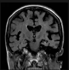
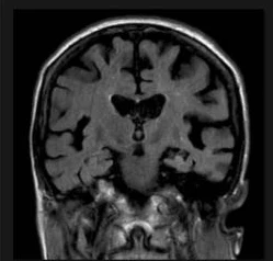
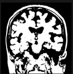
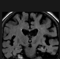
Then: bounding box of the largest contour, resize, back to RGB, normalization to mean 0.5 and standard deviation 0.5 per channel.
II.B · Preprocessing · Interactive
Otsu Lab: Find the Head, Crop the Frame
Runs in your browser on the Fig. 1 images. Otsu picks the threshold that maximizes the variance between the dark and bright pixel groups.
II.C · Model Architecture
A Stacked Ensemble with a Meta-Learner
DenseNet201torchvision · 4 outputs
ResNet50torchvision · 4 outputs
Dropout 0.4 → Linear to 512 → ReLU → BatchNorm → Dropout 0.2 → Linear to 4 classes.
A fixed vote treats all models alike. The MLP learns patterns in their joint outputs, e.g. which model to trust for which class.
DenseNet201 reuses features from all earlier layers.
ResNet50 eases training of deep networks; EfficientNet-B0 scales depth, width and resolution together.
II.D · Training
Training Setup
| Setting | Value |
|---|---|
| Hardware | NVIDIA GeForce RTX 3050, CUDA 11.8 |
| Framework | PyTorch with automatic mixed precision |
| Batch size | 8, shuffled |
| Loss | cross-entropy, label smoothing 0.1 |
| Optimizer | AdamW, learning rate 1e-4 |
| Schedule | cosine annealing |
| Epochs | 10 |
autocast runs the forward pass in half precision where safe; GradScaler scales the loss so small gradients do not underflow.
Targets of 0.9 instead of 1.0 discourage over-confident outputs, which also helps the meta-learner.
III.B · Fig. 3
Training Progress of the Ensemble
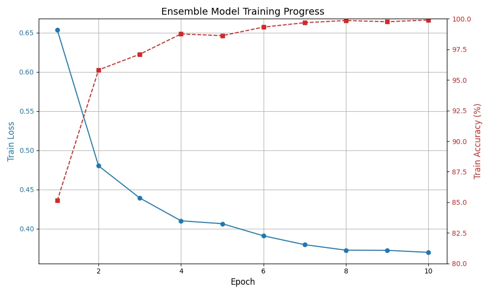
- Loss falls from about 0.65 to about 0.37; with label smoothing it cannot reach zero.
- Accuracy jumps after epoch 1 and approaches 100% by epoch 10.
- Ten epochs are enough because all three base models start from pretrained weights.
III.B · Table 1 · Interactive
Individual Models vs. the Ensemble
Weighted F1: DenseNet201 0.987 · ResNet50 0.988 · EfficientNet-B0 0.991 · ensemble 0.998. The axis starts at 0.97; hover a row for exact values.
III.B · Fig. 2 · Interactive
Where the Ensemble Still Errs
Hover or tap a cell. Rows are true labels, columns predictions.
- All 140 tumor-free scans are recognized.
- Most errors involve meningioma, in both directions.
- Off-diagonal cells hold 2 to 9 scans each.
IV · Discussion
Why It Works
Each CNN makes different mistakes; the meta-learner combines their strengths, e.g. ResNet50's glioma precision and EfficientNet-B0's no-tumor score.
Otsu thresholding and ROI cropping remove empty background, so more pixels show the brain.
BRISC's diverse, consistent, expertly annotated scans support robust training.
Mixed precision lets three CNNs train on a 6 GB laptop GPU, relevant for resource-limited clinics.
V · Conclusion
Conclusion
- Stacking EfficientNet-B0, DenseNet201 and ResNet50 with an MLP meta-learner reaches a weighted F1 of 0.998 on the BRISC test set.
- It beats every base model; EfficientNet-B0 is the strongest single model (0.991).
- Preprocessing and data quality matter as much as the architecture.
- Mixed precision keeps the cost of three networks manageable on modest hardware.
V · Conclusion
Check Questions
- What does the meta-learner receive as input, and what does it output?
- How is a stacked ensemble different from majority voting?
- In the Otsu lab, what happens to the crop when the threshold is far too low?
- Why does the training loss stay above zero even at almost 100% accuracy?
- Which confusion in Fig. 2 would worry a clinician most, and why?
Show answers
- The 12 concatenated outputs of the three base models (4 classes each); it outputs scores for the 4 classes.
- Voting combines outputs with a fixed rule; stacking trains a model that learns how much to trust each base model.
- Background noise joins the foreground, the largest region grows to the whole frame and the crop removes nothing.
- Label smoothing (0.1) sets targets below 1, so the cross-entropy cannot reach zero.
- The 9 meningiomas predicted as no tumor: a missed tumor delays treatment.
References
Selected References
- Fateh, A. et al. (2025). BRISC: Annotated dataset for brain tumor segmentation and classification with Swin-HAFNet. arXiv:2506.14318.
- Jader, R. F., Kareem, S. W., Awla, H. Q. (2024). Ensemble deep learning technique for detecting MRI brain tumor. Appl. Comput. Intell. Soft Comput., 6615468.
- Asif, S., Zhao, M., Chen, X. (2023). BMRI-NET: A deep stacked ensemble model for multi-class brain tumor classification from MRI images. Interdiscip. Sci. Comput. Life Sci., 15, 499–514.
- Çetin-Kaya, Y., Kaya, M. (2024). A novel ensemble framework for multi-classification of brain tumors using magnetic resonance imaging. Diagnostics, 14, 383.
- Tandel, G. S. et al. (2023). Role of ensemble deep learning for brain tumor classification in multiple magnetic resonance imaging sequence data. Diagnostics, 13, 481.
See the full paper for the complete reference list. Figures on these slides are from the paper.