Research Article · IEEE Access · Vol. 14 · 2026

Enhancing Radar PPI-Based Maritime Object Detection Using Hybrid Preprocessing and Deep Learning Approach

Sercan Külcü

Department of Computer Engineering, Giresun University, Türkiye

Radar PPI350 simulated framesPreprocessing labKernel sizeP2 layer Area-aware loss5 YOLO modelsLatencyLight backbonesReal DAAN data

doi: 10.1109/ACCESS.2026.3715472 · Use ← → or Space to navigate, F for full screen

Summary

At a Glance

Off-the-shelf detectors miss small, low-contrast buoys in radar PPI images. This study combines radar-specific preprocessing with two small-object changes to YOLO, then checks whether the gains survive on real radar.

Simulated, best mAP500.958YOLOv12s + P2 + Loss

Buoy mAP50-950.321 → 0.612YOLOv12s, raw → full

Real DAAN mAP500.698 → 0.922raw → full configuration

Missed targets−77%1,339 → 311 on DAAN

Preprocessing

HSV segmentation, adaptive binarization and morphological closing clean the radar frame.

Architecture

A high-resolution P2 head and an area-aware loss for boxes under 8 × 8 px.

Validation

Five YOLO models on simulator data, then external tests on real Baltic Sea radar.

1 · Introduction

Why Radar PPI Images Are Hard for Detectors

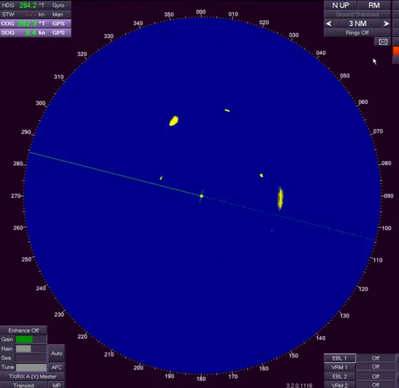
Real X-band radar PPI screen capture from the DAAN dataset — A real PPI screen (DAAN, Fig. 9)

The Plan Position Indicator shows radar returns as a 2-D polar map around the own ship: the cornerstone of radar navigation in fog, at night and in heavy traffic.

Not a photograph: grey-level intensity instead of colour and edges, diffuse boundaries.
Clutter that looks like targets: sea clutter, speckle noise, low SNR, multipath.
Small, weak targets: buoys cover a few pixels and are easily missed or loosely boxed.
The gap: classic fixes (thresholding, morphology) are rarely built into end-to-end deep pipelines, and new YOLO variants are rarely tested on radar PPI.

1 · Introduction

Four Contributions

High-resolution P2 layer

Added to selected YOLO models to keep fine spatial detail for small, low-contrast objects.

Area-aware loss

Box losses of objects smaller than 8 × 8 px are weighted up, so safety-critical buoys are not under-learned.

Five-model comparison

YOLOv5s, v8s, v10s, v11s and v12s on the same 350-frame simulated dataset, raw and preprocessed.

Real-world validation

External tests on the DAAN marine radar dataset, with an analysis of simulated-to-real transfer.

Unlike studies that address one component (clutter suppression, lightweight detection, segmentation or tracking), this work integrates preprocessing, model evaluation, P2, loss design, light backbones and real-data validation in one pipeline (Table 1).

2 · Methodology · Table 2

A 350-Frame Simulated Radar Dataset

Generated with the Wärtsilä NTPro 5000® bridge simulator.
Screenshots at set intervals from a ~2-hour recording, not consecutive video frames, so scenes are diverse.
Captured at 1280 × 1280, resized to 640 × 640.
Three classes: fixed (buoys), target (moving vessels), landmass (coastline).
Auto-labelled, then manually cross-validated.
Split 70 / 20 / 10%: 5,204 / 1,730 / 913 instances.

Fixed 13.9%Target 38.5%Landmass 47.6%

Buoys are the rarest class (724 training instances) and the smallest, yet the most critical for safe navigation.

2 · Methodology · Algorithm 1

A Four-Step Preprocessing Pipeline

1 · HSVRGB → hue, saturation, value: colour separated from intensity

→

2 · Colour maskkeep the narrow yellow hue range of strong echoes (Eq. 1)

→

3 · Adaptive binaryGaussian-weighted local threshold, 11 × 11 (Eqs. 2–3)

→

4 · Closingdilation then erosion, 11 × 11 kernel (Eq. 4)

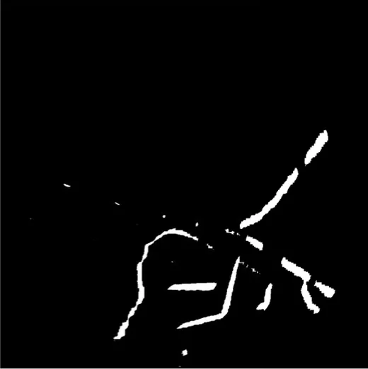
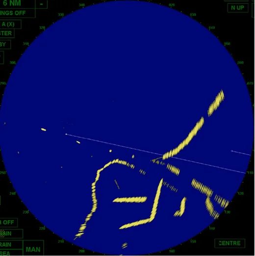
processedraw

Drag the divider to compare the raw frame and the result (Fig. 3).

The HSV thresholds are stable because commercial radar displays use fixed colour lookup tables: strong echoes always fall in a narrow yellow band.

The result keeps high-intensity echoes, joins their fragments and removes the disc, range rings and interface text.

2 · Methodology · Interactive

Preprocessing Lab: Run the Pipeline Yourself

Kernel

Runs in your browser on the Fig. 3 frame. The hue range and threshold offset are chosen for this demo; the paper's exact thresholds were set empirically and are not listed.

2 · Methodology · Fig. 2

Choosing the Closing Kernel

Kernel

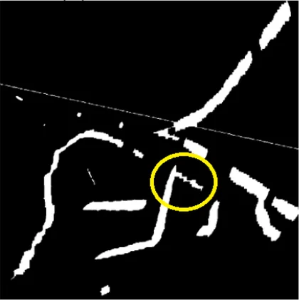
< 7 × 7

gaps remain
split detections

> 11 × 11

over-smoothing
separate echoes merge

11 × 11 is dataset-specific: echo thickness, display scale and clutter differ between radars, so it should be re-tuned for other systems.

2 · Methodology · Algorithm 2

From Contours to YOLO Labels

External contours of the processed frame are boxed; the box area A = w × h decides the initial class.

Fixed (buoy)

A < T_fixed: small, stationary echoes

Target (vessel)

T_fixed ≤ A < T_target: moderate, moving echoes

Landmass

A ≥ T_target: large, stable regions

(x_c, y_c, w_n, h_n) = ( (x + w/2) / W, (y + h/2) / H, w / W, h / H ) (5)

Caveat. Area ignores range, aspect angle and echo spreading: a distant vessel can look as small as a buoy. Area-only labelling is an initial annotation aid; every label was manually checked and corrected.

2 · Methodology

Five YOLO Generations

Model	Key idea	Expected effect on radar
YOLOv5s	CSPDarknet53 + PANet, anchor-based head	solid baseline; fixed anchors fit variable echo shapes poorly
YOLOv8s	anchor-free, decoupled heads	better localization of scattered, low-contrast targets
YOLOv10s	ELAN backbone, efficient anchor-free design	aimed at resource-constrained, real-time use
YOLOv11s	refined v8 backbone / neck, SPPF, better training	robust features and generalization
YOLOv12s	attention-centric: R-ELAN, Area Attention (A2C2f)	larger effective receptive field, focus on informative regions

L_YOLO = λ_boxL_box + λ_objL_obj + λ_clsL_cls (7)

Box loss uses Complete IoU; every model was trained with the same hyperparameters.

2 · Methodology · Fig. 4, Eqs. (8)–(10)

Seeing Smaller: the P2 Feature Layer

YOLOv12s architecture with the added P2 detection branch — YOLOv12s + P2 (Fig. 4)

F_P2 = Concat( Upsample(F_P3, 2), B_P2 ), D_P2 = A2C2f(F_P2)

Object size

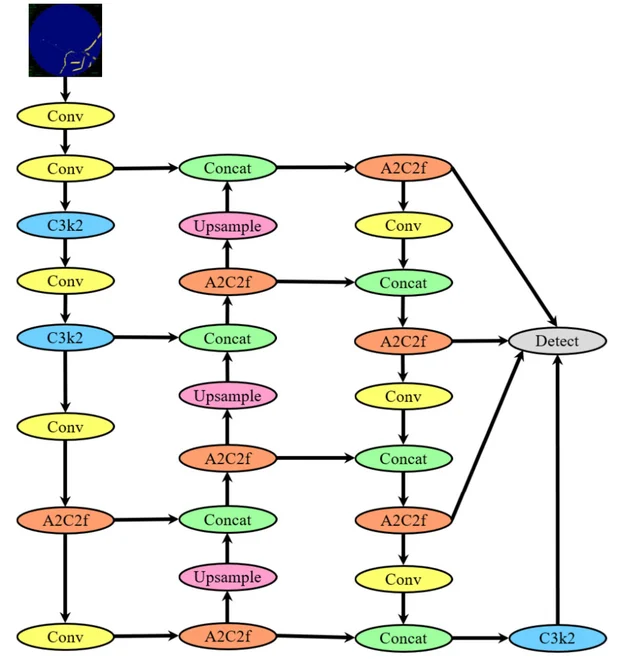
The head now predicts at P2/4, P3/8, P4/16 and P5/32. At 640 px input, P2 is a 160 × 160 map: an 8 × 8 px buoy spans 2 × 2 cells instead of a quarter of a P5 cell.

2 · Methodology · Eqs. (11)–(12)

Teaching the Model to Care About Small Objects

L_area-aware = Σ_i w_i · ( L_IoU,i + L_DFL,i ), w_i = 2.0 if A_i < 8 × 8, else 1.0

Box width

Box height

Weight

Dashed square: the 8 × 8 threshold, about the median buoy size. Loss share is a toy estimate: training instances from Table 2, half of the buoy boxes taken as small, equal per-box loss.

3 · Results

Training Configuration and Metrics

Framework	Ultralytics 8.3.170, PyTorch 2.9
Training GPU	RTX 5070 (12 GB)
Input / batch	640 px / 16
Epochs	250 (mosaic off for last 10)
Optimizer	AdamW, lr 0.001429, momentum 0.9
Loss gains	box 7.5 (CIoU), cls 0.5, dfl 1.5
Augmentation	flip 0.5, scale 0.5, translate 0.1, HSV h/s/v 0.015/0.7/0.4

P = TP / (TP + FP) R = TP / (TP + FN)

mAP50: mean AP over the three classes at IoU 0.5.

mAP50-95: also averaged over IoU 0.50, 0.55 … 0.95, a stricter localization test.

Latency was measured separately on a laptop RTX 3050 (6 GB), 640 × 640 input.

3 · Results · Tables 3–5

Results Explorer

Stage

Class

Metric

3 · Results · Tables 3–5

Where the Gains Come From: the Fixed Class

Metric

YOLOv8sYOLOv12s

Preprocessing

The largest single step: YOLOv12s buoy mAP50-95 0.321 → 0.503.

P2 layer

Finer features: 0.503 → 0.595.

Area-aware loss

Mainly recall: YOLOv8s buoy recall 0.843 → 0.936.

3 · Results · Fig. 7

Detection Outputs: Raw vs Preprocessed

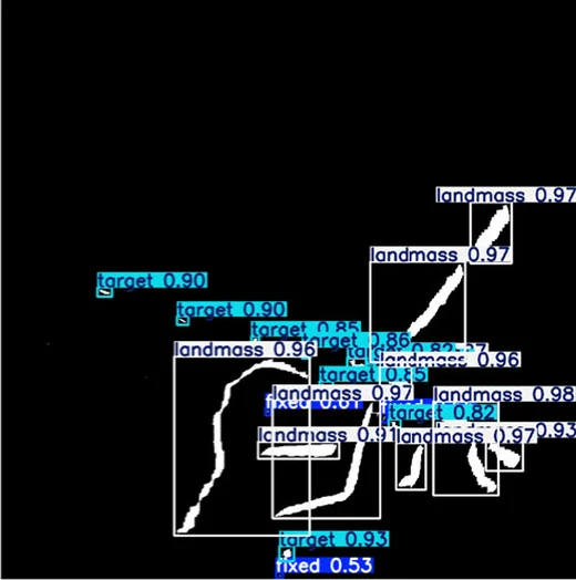
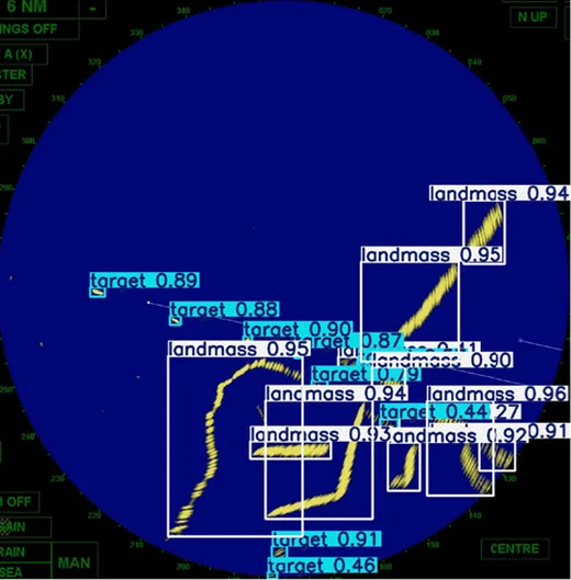
preprocessedraw

Predicted boxes with confidence scores on the same scene.

On the raw frame, boxes overlap heavily around the coastline and small echoes compete with clutter.
On the preprocessed frame the echoes are isolated, so landmass, target and fixed objects are separated more cleanly.

Overall YOLOv12s: mAP50 0.850 → 0.917, recall 0.836 → 0.904 from preprocessing alone.

3 · Results · Tables 6–7

Inference Latency

Images

standardP2 variantsdot: mean · band: ± sd · line: min–max

Standard models run faster than P2 variants, the expected cost of an extra detection scale. The area-aware loss changes training, not the inference graph, so its effect on latency is small.

3 · Results · Table 8

Model Complexity (click a header to sort)

Model	Configuration	Layers	Params (M)	GFLOPs
YOLOv5s	Standard	153	9.12	24.0
YOLOv8s	Standard	129	11.14	28.7
YOLOv10s	Standard	234	8.07	24.8
YOLOv11s	Standard	181	9.43	21.6
YOLOv12s	Standard	272	9.25	21.5
YOLOv5s	Optimized	84	9.11	23.8
YOLOv8s	Optimized	72	11.13	28.4
YOLOv10s	Optimized	106	7.22	21.4
YOLOv11s	Optimized	100	9.41	21.3
YOLOv12s	Optimized	159	9.23	21.2
YOLOv8s + P2	Standard	160	10.64	37.0
YOLOv12s + P2	Standard	327	9.38	28.3
YOLOv8s + P2	Optimized	90	10.63	36.6
YOLOv12s + P2	Optimized	189	9.36	27.8

"Optimized" = inference-time graph simplifications such as layer fusion. P2 barely changes the parameter count but raises GFLOPs (YOLOv8s 28.7 → 37.0): high-resolution maps are expensive to process.

3 · Results · Table 9

Lightweight Backbones: Accuracy vs Cost

Y axis

YOLOlightweight backbonehover for params and latency

YOLO models

Best accuracy: YOLOv12s mAP50 0.917, YOLOv8s mAP50-95 0.762.

ShuffleNetV2

Fastest and lightest: 1.8 GFLOPs, 9.1 ms, small accuracy cost.

GhostNet

Best balance: 0.751 mAP50-95 with 5.2 M params and 7.1 GFLOPs.

4 · Real-Data Validation · Figs. 9–10

The Real Test: DAAN Marine Radar Dataset

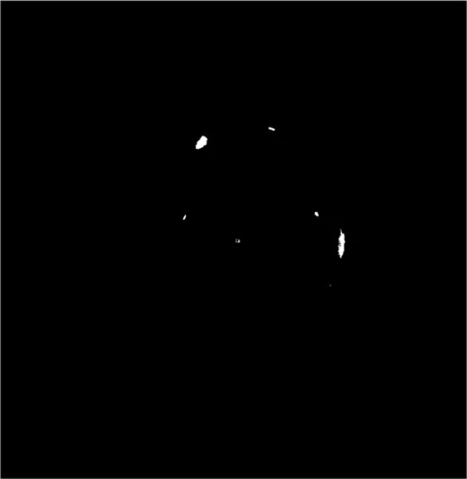
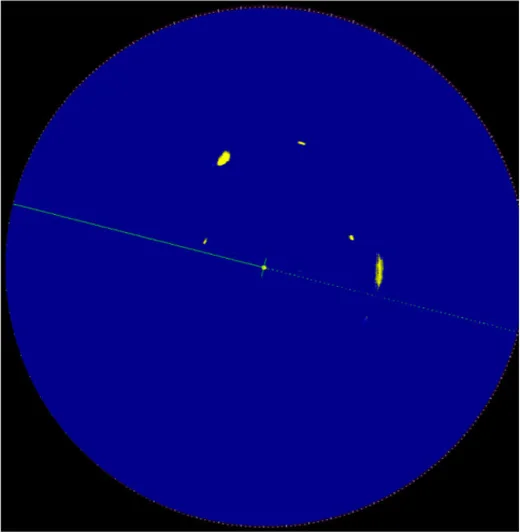
preprocessedcropped

Public DLR dataset recorded in the Baltic Sea: X-band radar screen captures at ~1 Hz from a moving own ship, with AIS reference tracks.
Four vessels, own-ship motion, wake trails, varied encounter geometry.
3 NM range, no MTI or Doppler: clutter and echo distortion are preserved.
AIS gives positions, not echo shapes, so labels come from a contour pipeline on the images with human checks.
Never used in training: a true cross-domain test (platform, clutter, rendering).

4 · Real-Data Validation · Table 10

Do the Gains Transfer to Real Radar?

missed detections (FN)false alarms (FP)

Configuration	TP	FP	FN	mAP50	mAP50-95
Raw	3301	41	1339	0.6983	0.6750
Preprocessed	4296	230	344	0.9149	0.7243
Preprocessed + P2	4306	315	334	0.9169	0.7406
Preprocessed + P2 + Loss	4329	315	311	0.9218	0.7451

False alarms rise (41 → 315), but missed detections fall far more (1,339 → 311): a better trade-off for navigation safety.

4 · Real-Data Validation · Fig. 11

Predictions on a Real Frame

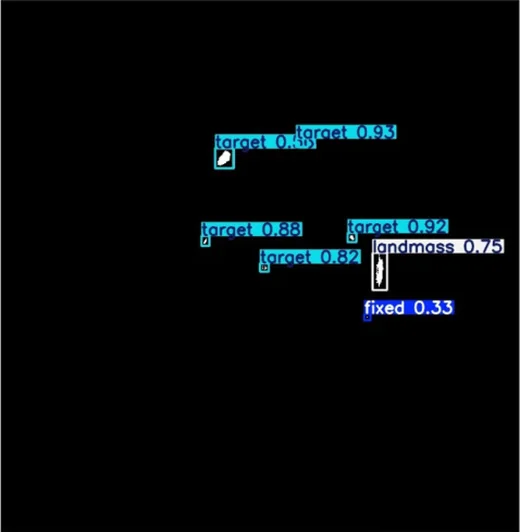
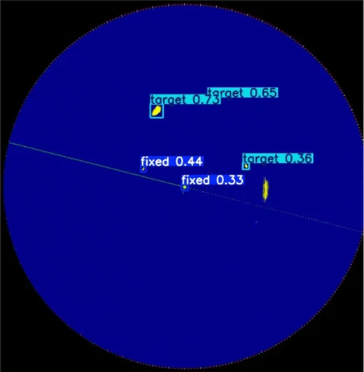
Predictions of YOLOv12s with P2 and area-aware loss on the preprocessed frame

Predictions of YOLOv12s trained on raw images

full modelraw model

Raw model: YOLOv12s trained on raw frames finds a few targets with low confidence (0.36–0.73).

Full model: YOLOv12s + P2 + area-aware loss on the preprocessed frame finds more targets with higher confidence (0.82–0.93).

The simulator has three classes but DAAN only has vessels, so some clutter points come out as "fixed" and some distorted echoes as "landmass".

5 · Discussion

Discussion and Limitations

Complementary parts

Preprocessing makes buoys visible, P2 keeps them resolvable, the loss keeps them from being ignored. Larger classes do not suffer.

Accuracy has a price

P2 variants are slower and need more GFLOPs; lightweight backbones such as GhostNet are a real-time alternative.

Evidence of transfer

On DAAN the full configuration reduces misses and finds weak echoes, suggesting it learns radar structure, not simulator artefacts.

Limits

Simulated and display-captured images; one external domain; HSV thresholds and the 11 × 11 kernel depend on the display and radar.

6 · Conclusion

Conclusion and Future Work

Radar-specific preprocessing lifts every YOLO model, most of all on small, low-contrast buoys.
P2 + area-aware loss: YOLOv8s reaches 0.957 / 0.813 and YOLOv12s 0.958 / 0.812 (mAP50 / mAP50-95) on the simulated set.
On real DAAN radar the full configuration reaches 0.922 mAP50 and 0.745 mAP50-95, up from 0.698 and 0.675.
The approach supports reliable real-time situational awareness for autonomous maritime navigation.

Next steps

Larger real-world radar datasets from multiple platforms
Domain adaptation for cross-radar generalization

6 · Conclusion

Check Questions

Why can a fixed HSV range isolate echoes reliably on commercial radar displays?
What goes wrong with a closing kernel that is too small, and with one that is too large?
An 8 × 8 px buoy at 640 px input: how many cells does it cover on P2 and on P5?
Why does the area-aware loss mostly raise recall rather than precision?
On DAAN, false positives rise from 41 to 315. Why is the full configuration still preferred?

Show answers

The images are captured after display processing, which maps strong echoes to a fixed yellow through colour lookup tables.
Too small leaves echoes fragmented (split detections); too large over-smooths and merges independent reflections.
P2 (stride 4): 2 × 2 cells. P5 (stride 32): 0.25 × 0.25, a quarter of one cell.
Small boxes get twice the weight, so weak buoy echoes are no longer ignored during training: fewer misses.
Missed detections drop from 1,339 to 311; for navigation a missed vessel is more dangerous than an extra alarm.

References

Selected References

J. S. Fowdur, M. Baum, F. Heymann, "Real-world marine radar datasets for evaluating target tracking methods," Sensors, vol. 21, no. 14, 4641, 2021.
S. Külcü, "Radar image-based object detection and tracking for autonomous surface vehicles," Turkish J. Maritime Mar. Sci., vol. 12, no. 1, pp. 35–47, 2026.
Y. Tian, Q. Ye, D. Doermann, "YOLOv12: Attention-centric real-time object detectors," 2025.
A. S. Alamoush, A. I. Ölçer, "Maritime autonomous surface ships: Architecture for autonomous navigation systems," JMSE, vol. 13, no. 1, 122, 2025.
Wärtsilä NTPro 5000 bridge simulator; DAAN marine radar dataset, German Aerospace Center (DLR).

The paper lists 46 references. Figures are reproduced from the article, published under a CC BY 4.0 licence.

Thank You

Enhancing Radar PPI-Based Maritime Object Detection Using Hybrid Preprocessing and Deep Learning Approach

How to cite: Külcü, S. (2026). Enhancing Radar PPI-Based Maritime Object Detection Using Hybrid Preprocessing and Deep Learning Approach. IEEE Access, 14, 111715–111730. doi:10.1109/ACCESS.2026.3715472

sercan.kulcu@giresun.edu.tr · All publications

1 / 1